Photometry of HAT-P-36P

Kari Nilsson
Finnish Center for Astronomy with ESO (FINCA)
University of Turku, Finland
Feb 2020

1. Introduction

HAT-P-36b is an exoplanet oribiting its parent star with an inclination of nearly 90 degrees, which makes it transit (go in front of) its parent star causing a small "eclipse". The transits can be accurately predicted.

These data of the star HAT-P-36 (V = 12.26) were obtained at the Tuorla 1.03 meter telescope through the R-band filter by Sepideh Sadegi and Kari Nilsson in April 10-11, 2016. There are 249 images in the series, each with 30 seconds of exposure.

The images have been already reduced and ready to measure. The photometry will be done on differential mode, i.e. the brightness of HAT-P-36 is compared to the brightness of a neary star, which mostly eliminates instrumental and atmospheric effects.

2. Goals

During this exercise you will

1. Measure the light curve of HAT-P-36 turing transit and determine the depth of the eclipse.


2. Make some test how the light curve is affected by changes in the measurement parameters.

Everything will be done in tube.utu.fi using IRAF.

3. Practical work

3.1 Copy the data

The data are in tube.utu.fi in /coursedata. There are 249 fits files and 249 coordinate files.

1. Start up IRAF as described here. If you are starting IRAF for the first time, follow the instructions to create a new project.
   
   
2. You shoud now have 3 windows open: linux xterm, IRAF xgterm and ds9. Go to the linux xterm and make sure you are in the right directory (iraf), by issuing

   $ pwd

   Copy the data

   $ cp /coursedata/hatit/* .

   3.2 Take a look at the images

   Display one of the images on ds9 to see everything works and to get an idea of the data, e.g.

   ecl> display HAT-P-36b-0113R_reduced.fits 1
   

   you should see something like this :

   
   

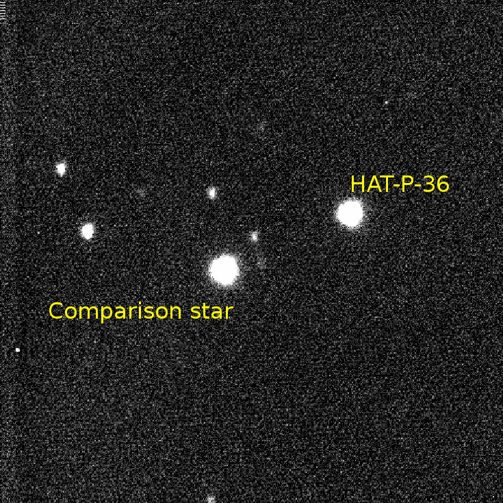
   A lot of info on any image can be obtained with

   ecl> imhead HAT-P-36b-0113R_reduced.fits l+
     

   where l+ means "long", i.e. show more information. The output should be:

   BSCALE  =   1.0
   BZERO   =   0.0
   DATE-OBS= '2016-04-10T23:58:48' /YYYY-MM-DDThh:mm:ss observation start, UT
   EXPTIME =   30.000000000000000 /Exposure time in seconds
   EXPOSURE=   30.000000000000000 /Exposure time in seconds
   SET-TEMP=  -20.000000000000000 /CCD temperature setpoint in C
   CCD-TEMP=  -20.013072750000003 /CCD temperature at start of exposure in C
   XPIXSZ  =   26.000000000000000 /Pixel Width in microns (after binning)
   YPIXSZ  =   26.000000000000000 /Pixel Height in microns (after binning)
   XBINNING=                    2 /Binning factor in width
   YBINNING=                    2 /Binning factor in height
   XORGSUBF=                    0 /Subframe X position in binned pixels
   YORGSUBF=                    0 /Subframe Y position in binned pixels
   READOUTM= 'Monochrome' /        Readout mode of image
   IMAGETYP= 'Light Frame' /       Type of image
   FOCALLEN=  0.00000000000000000 /Focal length of telescope in mm
   APTDIA  =  0.00000000000000000 /Aperture diameter of telescope in mm
   APTAREA =  0.00000000000000000 /Aperture area of telescope in mm^2
   SBSTDVER= 'SBFITSEXT Version 1.0' /Version of SBFITSEXT standard in effect
   SWCREATE= 'MaxIm DL Version 6.12 160429 0PX4F' /Name of software
   SWSERIAL= '0PX4F-3TNTK-EJMN9-FVJ1F-WY0KM-4X' /Software serial number
   SITELAT = '00 00 00' /          Latitude of the imaging location
   SITELONG= '00 00 00' /          Longitude of the imaging location
   JD      =   2457489.4991666665 /Julian Date at start of exposure
   OBJECT  = 'HAT-P-36b'
   TELESCOP= '        ' /          telescope used to acquire this image
   INSTRUME= 'Apogee USB/Net'
   OBSERVER= '        '
   NOTES   = '        '
   FLIPSTAT= '        '
   SWOWNER = 'Kari Nilsson' /      Licensed owner of software   
     

   3.3 Measure the FWHM if the stellar profile

   Measure the FWHM by typing

   ecl> imexamine image.fits
     

   Where image.fits is one of the images. Move cursor over a star and press r. You should get a radial plot of the star. Of the three rightmost values in the lower right corner of the plot, choose the middle one as your estimate for the FWHM.

   3.4 Edit IRAF parameters of phot

   Enter the Daophot package, which contains the photometry routines.

   ecl> noao
   
   ecl> digiphot
   
   ecl> daophot
   

   In this exercise you will use the phot task to perform aperture photometry of HAT-P-36 and a nearby star. In addition to phot itself, you will need to edit the parameters of four other tasks, datapars, centerpars, fitskypars and photpars
   
   1) Make a text file containing a list of images, e.g. by

   $ ls *reduced*.fits > hatit
   

   The image list is now in a file called hatit.
   
   2) Type

   ecl> epar phot
   

   And edit the parameters to

   							      
           image = "@hatit"        Input image(s)
          coords = "default"       Input coordinate list(s) (default: image.coo.?)
          output = "default"       Output photometry file(s) (default: image.mag.?
         skyfile = ""              Input sky value file(s)
       (plotfile = "")             Output plot metacode file
       (datapars = "")             Data dependent parameters
     (centerpars = "")             Centering parameters
     (fitskypars = "")             Sky fitting parameters
       (photpars = "")             Photometry parameters
    (interactive = no)             Interactive mode?
       (radplots = no)             Plot the radial profiles?
      (icommands = "")             Image cursor: [x y wcs] key [cmd]
      (gcommands = "")             Graphics cursor: [x y wcs] key [cmd]
          (wcsin = )_.wcsin)       The input coordinate system (logical,tv,physica
         (wcsout = )_.wcsout)      The output coordinate system (logical,tv,physic
          (cache = )_.cache)       Cache the input image pixels in memory?
         (verify = )_.verify)      Verify critical phot parameters?
         (update = )_.update)      Update critical phot parameters?
        (verbose = )_.verbose)     Print phot messages?
       (graphics = )_.graphics)    Graphics device
        (display = )_.display)     Display device
           (mode = "ql")           
   	

   Note that the just created list hatit is used as input. The coords is set to "default", which makes IRAF to look for a text file with a specific name, image.coo.N, where N is a running number starting from zero. These coordinate files have the (x,y) pixel positions of each target you want to measure.

   In this case there are only two targets, so the coordinate files have two lines. These files are kindly provided by your friendy instructor, who expects only mild worship in return.
   
   When you are ready close by ctrl-d.
   
   3) Type

   ecl> datapars
   

   (no need to type epar here, which is strange, but that's how it is) and edit to

          (scale = 1.)             Image scale in units per pixel
        (fwhmpsf = 5.)             FWHM of the PSF in scale units
       (emission = yes)            Features are positive?
          (sigma = 0.)             Standard deviation of background in counts
        (datamin = INDEF)          Minimum good data value
        (datamax = INDEF)          Maximum good data value
          (noise = "poisson")      Noise model
        (ccdread = "")             CCD readout noise image header keyword
           (gain = "")             CCD gain image header keyword
      (readnoise = 8.)             CCD readout noise in electrons
          (epadu = 2.3)            Gain in electrons per count
       (exposure = "")             Exposure time image header keyword
        (airmass = "")             Airmass image header keyword
         (filter = "")             Filter image header keyword
        (obstime = "")             Time of observation image header keyword
          (itime = 1.)             Exposure time
       (xairmass = INDEF)          Airmass
        (ifilter = "INDEF")        Filter
          (otime = "INDEF")        Time of observation
           (mode = "ql")      
   

   Here we mainly input the FWHM of the data and the readout noise and the gain of the camera so that IRAF can compute the noise properly.
   
   4) Type

   ecl> centerpars
   

   and edit to

       (calgorithm = "centroid")     Centering algorithm
           (cbox = 15.)            Centering box width in scale units
     (cthreshold = 0.)             Centering threshold in sigma above background
     (minsnratio = 1.)             Minimum signal-to-noise ratio for centering alg
       (cmaxiter = 10)             Maximum iterations for centering algorithm
       (maxshift = 10.)            Maximum center shift in scale units
          (clean = no)             Symmetry clean before centering
         (rclean = 1.)             Cleaning radius in scale units
          (rclip = 2.)             Clipping radius in scale units
         (kclean = 3.)             K-sigma rejection criterion in skysigma
       (mkcenter = no)             Mark the computed center
           (mode = "ql")  
   

   Here we tell IRAF the we want to find the position of the star by the "centroid" algorithm, which basically calculates the "center of weight" of the light distribution (imagine the pile of photons a mass and you need to find the balance point of that mass distribution).

   The cbox parameter tells IRAF the size of the box it should use for centering. Any size close to about 2 times the FWMH of the stellar profile will do.

   Set the maxshft to 1-2 times the FWHM to avoid unnecesssary error messages.

   5) Type

   ecl> fitskypars
     

   and edit to

     (salgorithm = "mode")         Sky fitting algorithm
        (annulus = 30.)            Inner radius of sky annulus in scale units
       (dannulus = 10.)            Width of sky annulus in scale units
       (skyvalue = 0.)             User sky value
       (smaxiter = 10)             Maximum number of sky fitting iterations
        (sloclip = 0.)             Lower clipping factor in percent
        (shiclip = 0.)             Upper clipping factor in percent
       (snreject = 50)             Maximum number of sky fitting rejection iterati
      (sloreject = 3.)             Lower K-sigma rejection limit in sky sigma
      (shireject = 3.)             Upper K-sigma rejection limit in sky sigma
          (khist = 3.)             Half width of histogram in sky sigma
        (binsize = 0.1)            Binsize of histogram in sky sigma
         (smooth = no)             Boxcar smooth the histogram
          (rgrow = 0.)             Region growing radius in scale units
          (mksky = no)             Mark sky annuli on the display
           (mode = "ql")             
       

   Here we set the region used to extract the sky brightness, which will subtracted from each pixel value within the aperture. The sky extraction ragion is a circular ring around the target with an inner radius of annulus and width of dannulus.

   Parameter annulus should be set so that the ring is as near as possible to the target without significant amount of target light entering the ring.

   For annulus 10-15 pix is usually a good value. Both annulus and dannulus should be set so that no bright targets enter the sky ring (faint targets are filtered out by IRAF). On the other hand, you should keep them as close to the target as possible in order to get a good estimate of the sky brightness in the aperture.

   6) Finally, type

   ecl> photpars
     

   and edit to

        (weighting = "constant")     Photometric weighting scheme
      (apertures = "3,10,25")           List of aperture radii in scale units
           (zmag = 25.)            Zero point of magnitude scale
        (mkapert = no)             Draw apertures on the display
           (mode = "ql")  
     

   Parameter apertures is the most crucial parameter of the whole process. Setting it too low or too high will result in increased noise in the light curve. The optimal value is 1.5-2 times the FWHM. Here we test three values, too low, optimal (which is not necesarily 10 pix, so you need to experiment a bit) and too high.

   3.5 Run phot

   It's time to do the photometry. Cross your fingers and type

   ecl> phot
       

   IRAF will as a multitude of questions, but if you set up everything correctly above, you just need to press enter fo each question.

   The screen will flood with output for a while. After phot finishes, you should have 249 files image.mag.1. These are just text files with the results at the bottom:

   HAT-P-36b-0115R_reduced375.100   279.700   1     HAT-P-36b-0115R_reduced1      \
      375.488    279.659    0.388   -0.041  0.005   0.006          0    NoError   \
      311.8127       16.35223       5.625587       2184   11       0    NoError   \
      1.             INDEF          INDEF                  INDEF                  \
      3.00     153722.       28.42374   144859.2      12.098 0.002 0    NoError  *\
      10.00    543678.5      314.3708   445653.7      10.878 0.001 0    NoError  *\
      25.00    1110037.      1963.364   497835.3      10.757 0.002 0    NoError  * 
   HAT-P-36b-0115R_reduced249.100   221.700   2     HAT-P-36b-0115R_reduced2      \
      247.649    222.377    -1.451  0.677   0.004   0.005          0    NoError   \
      314.2496       16.61773       6.882789       2191   5        0    NoError   \
      1.             INDEF          INDEF                  INDEF                  \
      3.00     242496.9      28.44734   233557.4      11.579 0.002 0    NoError  *\
      10.00    763566.4      314.4176   664760.8      10.443 0.001 0    NoError  *\
      25.00    1354803.      1963.351   737821.3      10.330 0.002 0    NoError  *
       

   On the left you see the apertures you just selected. On the right are the corresponding magnitudes.

   3.6 Plotting the light curve

   One way to extract the magnitudes into a single file is (in this example the 3.0 aperture results is type in a unix terminal (not in xgterm)

   $ find . -name '*.mag.*' -exec grep -H '3.00 ' {} \; > temp.txt
       

   This should extract the results of aperture 3.00 to a file called temp.txt, which should look like this approx:

    /HAT-P-36b-0241R_reduced.fits.mag.1:   3.00     89734.85      28.46094   82948.98      12.703 0.003 0    NoError  *\
   ./HAT-P-36b-0241R_reduced.fits.mag.1:   3.00     152978.6      28.42824   146066.       12.089 0.002 0    NoError  *\
   ./HAT-P-36b-0016R_reduced.fits.mag.1:   3.00     158010.9      28.60328   148589.8      12.070 0.002 0    NoError  *\
   ./HAT-P-36b-0016R_reduced.fits.mag.1:   3.00     251018.1      28.80891   241438.4      11.543 0.002 0    NoError  *\
   ./HAT-P-36b-0129R_reduced.fits.mag.1:   3.00     135839.8      28.44002   127046.7      12.240 0.002 0    NoError  *\
   ./HAT-P-36b-0129R_reduced.fits.mag.1:   3.00     213429.5      28.58903   204503.4      11.723 0.002 0    NoError  *\
   ./HAT-P-36b-0133R_reduced.fits.mag.1:   3.00     123418.2      28.63371   99802.05      12.502 0.003 0    NoError  *\
   ./HAT-P-36b-0133R_reduced.fits.mag.1:   3.00     186570.5      28.60643   163246.5      11.968 0.002 0    NoError  *\
   ./HAT-P-36b-0072R_reduced.fits.mag.1:   3.00     141657.       28.58454   132613.6      12.194 0.002 0    NoError  *\
   ./HAT-P-36b-0072R_reduced.fits.mag.1:   3.00     228032.4      28.48608   218954.8      11.649 0.002 0    NoError  *\
   ./HAT-P-36b-0172R_reduced.fits.mag.1:   3.00     138178.2      28.4653    129135.3      12.222 0.002 0    NoError  *\
   ./HAT-P-36b-0172R_reduced.fits.mag.1:   3.00     227682.6      28.41707   218495.2      11.651 0.002 0    NoError  *\
   ./HAT-P-36b-0032R_reduced.fits.mag.1:   3.00     141956.7      28.434     132732.4      12.193 0.002 0    NoError  *\
   ./HAT-P-36b-0032R_reduced.fits.mag.1:   3.00     224431.5      28.49857   215138.3      11.668 0.002 0    NoError  *\
    ./HAT-P-36b-0098R_reduced.fits.mag.1:   3.00     147498.2      28.53423   138472.5      12.147 0.002 0    NoError  *\
    etc...
       

   Now we have the magnitudes alternating between HAT-P-36 amd the comparison star. As in the example above, you will discover that the results are in wrong order, i.e. the first lines do no contain the results of the first image etc. To correct this type

   $ sort temp.txt > photometry_3.00.txt
       

   which will put the files in the correct order. Next, using your favorite editor/programming a small utility, edit photometry_3.00.txt to this format:

      12.185 0.002    11.660 0.002	
      12.144 0.002    11.613 0.002
      12.124 0.002    11.602 0.002
      12.196 0.002    11.649 0.002
      12.190 0.002    11.654 0.002
      12.084 0.002    11.554 0.002
      12.073 0.002    11.544 0.002
      12.222 0.002    11.694 0.002
      12.086 0.002    11.561 0.002
      12.074 0.002    11.534 0.002
      12.027 0.002    11.512 0.001
      12.175 0.002    11.664 0.002
      11.969 0.002    11.453 0.001
      etc...
         

   i.e. you have 4 columns : HAT-P-36 mag and error, comparison star mag and error.

   Next we need to extract the times of observation which are sadly not included in the mag files. Type in IRAF

   ecl> imhead HAT*.fits l+ > head.txt
       

   and in linux terminal

   $ grep DATE-OBS head.txt > times.txt
       

   Now times.txt contains the observing times. You need to edit this file too to remove unnecessary colums and combine times.txt with photometry_3.00.txt to make photometry_3.00.txt to look like this :

   2016-04-10T22:56:38   12.185 0.002    11.660 0.002
   2016-04-10T22:57:08   12.144 0.002    11.613 0.002
   2016-04-10T22:57:39   12.124 0.002    11.602 0.002
   2016-04-10T22:58:10   12.196 0.002    11.649 0.002
   2016-04-10T22:58:41   12.190 0.002    11.654 0.002
   2016-04-10T22:59:12   12.084 0.002    11.554 0.002
   2016-04-10T22:59:43   12.073 0.002    11.544 0.002
   2016-04-10T23:00:14   12.222 0.002    11.694 0.002
   2016-04-10T23:00:44   12.086 0.002    11.561 0.002
   2016-04-10T23:01:15   12.074 0.002    11.534 0.002
   2016-04-10T23:02:03   12.027 0.002    11.512 0.001
   2016-04-10T23:02:33   12.175 0.002    11.664 0.002
   2016-04-10T23:03:04   11.969 0.002    11.453 0.001
   2016-04-10T23:03:35   12.047 0.002    11.518 0.001
   2016-04-10T23:04:06   12.034 0.002    11.498 0.001
   2016-04-10T23:04:37   12.070 0.002    11.543 0.002
   2016-04-10T23:05:08   12.332 0.002    11.793 0.002
   etc...
       

   Next we plot the results, i.e. time versus the magnitude difference. Using gnuplot this can be achieved with

   $ gnuplot
   
   unset key
   set xdata time
   set timefmt "%Y-%m-%dT%H:%M:%S"
   set format x "%d.%m.\n%Y\n%H\"
   plot 'photometry_3.00.txt' u 1:($2-$4):(sqrt($3*$3+$5*$5)) w e pt 7
         

   Repeat this procedure for the other two apertures.

   4. Final report

   The final report should contain the following:

   1. Short introduction to the project.
   2. A description of steps taken and a justification for the parameter values (fwhm, aperture, sky rings, ...) chosen.
   3. The best light curve obtained and at least one example of a suboptimal one. Discuss the reasons why one curve is better than the other.
   4. Dou you see the eclipse? Give start time, end time and duration.
   5. If the eclipse is difficult to see, discuss why this might be.
   6. How does the observation compare with prediction? The latter can be found by searching the internet.